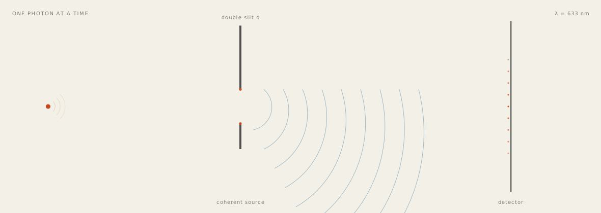
The double slit is usually introduced as a wave experiment. Run it with a source weak enough that only one photon is in the apparatus at a time, and the same pattern appears — dot by dot. No photon interferes with another photon. Each detection is a single event, and the pattern is what remains after many events.1
The experiment
A source illuminates a barrier with two narrow slits, separated by $d$, and a screen sits a distance $L$ away. With a bright source the screen shows fringes immediately. With a single-photon source and a detector that records individual arrivals, the fringes appear only after the detections accumulate. The apparatus is the same; the intensity is different.
Each detection has a position, never a trajectory. If the photon is detected at a particular $x$, no measurement in the apparatus says which slit it passed through. That absence of information is not a technical limitation; it is the condition for the pattern.
The pattern
The amplitude at the screen is the sum of the amplitudes from the two slits, and the probability is the square:
\[ I(x)\propto\left|\psi_{1}(x)+\psi_{2}(x)\right|^{2}. \]
For slit separation $d$ and screen distance $L$, the fringe spacing is
\[ \Delta x=\frac{\lambda L}{d}. \]
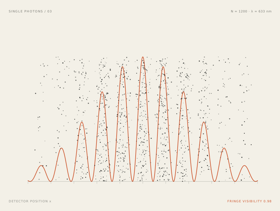
The envelope is set by the width of each slit. For $\lambda=633$ nm, $d=0.12$ mm and $L=1.2$ m, the spacing is about $6.3$ mm — large enough to see on a screen, small enough that alignment matters.
Which path
Now make the paths distinguishable. A polariser in one arm, a path marker, or a detector that records which slit the photon used will do. The interference term disappears, and the pattern becomes the sum of two single-slit envelopes:
\[ I(x)\propto\left|\psi_{1}(x)\right|^{2}+\left|\psi_{2}(x)\right|^{2}. \]
The trade is quantitative. Define the fringe visibility $V$ and the path distinguishability $D$. For a two-path experiment,
\[ V=\frac{I_{\max}-I_{\min}}{I_{\max}+I_{\min}}, \]
\[ V^{2}+D^{2}\le1. \]
Perfect path information means no fringes; perfect fringes mean no path information. The inequality, in this form due to Englert, is complementarity stripped of philosophy.
The quantum eraser is the subtle version. If the path information is erased before the photon is detected — for example, by a coincidence measurement on an entangled idler — the fringes can reappear in the coincidence counts. Nothing travels backwards in time, and no signal is sent. The erasure is a selection of sub-ensembles, and the price is the coincidence count.
What the lab measures
The conceptual experiment is clean; the apparatus is not. The source must be attenuated until the probability of two photons in the apparatus is small, but not so weak that the count rate becomes impractical. The slits must be aligned to a few microns. The detector has dark counts, and the source has a finite coherence length. A fringe pattern with low visibility is not a failed demonstration of quantum mechanics; it is a measurement of these imperfections.
Visibility is a fit parameter, not a count of bright and dark dots. Dark counts add a flat background and pull the minima up; a finite coherence length reduces the envelope. Reporting $V=0.98$ without saying how it was extracted is a habit worth breaking.2
The simulation
The interactive figure on the research page samples detections from the same intensity law. With which-path information off, the dots build fringes. With it on, the fringes disappear and the two envelopes remain. The point of the simulation is not to replace the experiment; it is to make the distinction between “the pattern” and “a single detection” visible at a glance.
The deeper question is the one I keep circling: a detector is a physical object, not an abstract “which-path” label. What happens to the field when the detector is switched on, and how does the back-action appear in the coincidence counts? That is a real experiment, not a thought experiment.
Revision history
- 10 Nov 2026 — Corrected a reference. The anticorrelation experiment is Grangier, Roger and Aspect, Europhys. Lett. 1, 173 (1986); the first version gave the wrong journal and author order. Added Englert's paper as the source of the inequality $V^{2}+D^{2}\le1$.
- 12 Oct 2026 — First published.
References
- R. P. Feynman, R. B. Leighton, and M. Sands, The Feynman Lectures on Physics, Vol. III, Ch. 1. online
- M. O. Scully and K. Drühl, “Quantum eraser: A proposed photon correlation experiment concerning observation and ‘delayed choice’ in quantum mechanics,” Phys. Rev. A 25, 2208 (1982). doi
- P. Grangier, G. Roger, and A. Aspect, “Experimental evidence for a photon anticorrelation effect on a beam splitter: A new light on single-photon interferences,” Europhys. Lett. 1, 173–179 (1986). doi
- B.-G. Englert, “Fringe visibility and which-way information: an inequality,” Phys. Rev. Lett. 77, 2154–2157 (1996). doi
- M. Born and E. Wolf, Principles of Optics, 7th ed. Cambridge University Press, 1999.